ccd_time
Command line options
This module is deprecated and not used any more!!!!
Usage: ccd_time [options]

Options:
  -h, --help            show this help message and exit
  -d FILE, --data_file=FILE
                        data file (default: data.dat)
  --fmax=FLOAT          Ignore frequencies above this value (default: None)
  --fmin=FLOAT          Ignore frequencies below this value (default: None)
  --data_format=FORMAT  Input data format, possible values are: rmag_rpha,
                        lnrmag_rpha, log10rmag_rpha, rmag_rpha,  rre_rim
                        rre_rmim, cmag_cpha, cre_cim, cre_cmim. "r" stands for
                        resistance/resistivity, and "c" stands for
                        conductance/conductivity (default: rmag_rpha)
  --data_weighting=SCHEME
                        Data weighting scheme to use. (default: re_vs_im)
  --lam0=FLOAT          Initial lambda for f-regularization (default: None)
  --f_lambda=FLOAT      Use a fixed lambda for the tau regularization
                        (default: None)
  -f FILE, --frequency_file=FILE
                        Frequency file (default: frequencies.dat)
  --ignore=STRING       Frequency ids to ignore, example:12,13,14. Starts with
                        index 0. (default: None)
  --ind_lams            Use individual lambdas for f-regularization (default:
                        False)
  --max_it=INT          Maximum number of iterations (default: 20)
  --norm=FLOAT          Normalize lowest frequency real part to this value
                        (default: None)
  -n INT, --nr_terms=INT
                        Number of polarization terms per frequency decade
                        (default: 20)
  -o DIR, --output=DIR  Output directory (default: results)
  --output_format=STRING
                        Output format(ascii| ascii_audit) (default:
                        ascii_audit)
  -i, --plot_its        Plot spectra of each iteration (default: False)
  --plot_lcurve=INT     Plot the l-curve for a selected iteration. WARNING:
                        This only plots the l-curve and does not use it in the
                        inversion process. Use -1 for last iteration.
                        (default: None)
  --plot_reg_strength   Plot regularization strengths of final iterations
                        (default: False)
  -p, --plot            Plot final iterations (default: False)
  --silent              Do not plot any logs to STDOUT (default: False)
  --tausel=STRATEGY     Tau selection strategy: data: Use data frequency
                        limits for tau selection data_ext (default): Extend
                        tau ranges by one frequency decade compared to the
                        'data' strategy. Factors can be set for the low and
                        high frequency by separating with a ',': LEFT,RIGHT,
                        e.g. '10,100' (default: data_ext)
  --tm_i_lambda=FLOAT   Fixed time regularization lambda for chargeabilities
                        m_i (default: 0)
  --trho0_lambda=FLOAT  Fixed time regularization lambda for rho0 (default: 0)
  --tw_mi               Use time-weighting (only in combination with
                        --tmi_first_order) (default: False)
  --tw_rho0             Use time-weighting (only in combination with
                        --trho0_first_order) (default: False)
  --times=FILE          Time index file (default: times.dat)
  --tmi_first_order     Use first order smoothing for m_i (instead of second
                        order smoothing) (default: False)
  --trho0_first_order   Use first order smoothing for rho_0 (instead of second
                        order smoothing) (default: False)
  --tmp                 Create the output in a temporary directory and later
                        move it later to its destination (default: False)
  -v, --version         Print version information (default: False)
Regularisation Parameters
The selection of appropriate regularisation parameter values is a non-trivial
task for ill-posed inverse problems. In the present case this particularly
holds for the time regularisation, which competes with the frequency
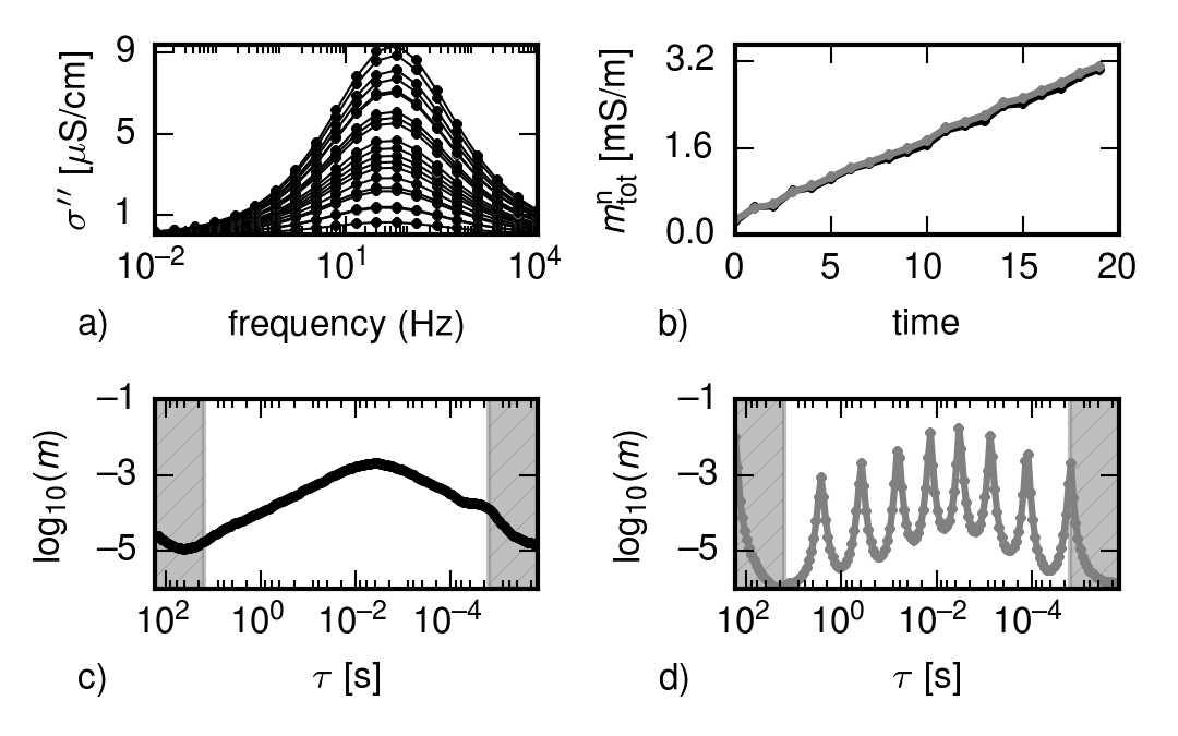
regularisation. The figure shows an example which highlights the importance of
appropriately balancing frequency and time regularisations. Unimodal SIP
responses were generated using the Cole-Cole model with increasing
chargeability over time (a). Based on these data, DDs were performed using two
different time regularisations: one characterised by reasonably balanced time
and frequency regularisation parameters, and one where time regularisation was
dominant. The resulting temporal evolution of  for both cases
is shown in (b) and the corresponding RTDs for time step 10 are shown in c and
d, respectively. Although the temporal evolution of is very
similar in both cases, a too strong time regularisation effectively neutralises
the frequency regularisation and leads to a highly fluctuating RTD (c).
for both cases
is shown in (b) and the corresponding RTDs for time step 10 are shown in c and
d, respectively. Although the temporal evolution of is very
similar in both cases, a too strong time regularisation effectively neutralises
the frequency regularisation and leads to a highly fluctuating RTD (c).
(figure taken from src/dd_single/characterisation/TooMuchTimeReg).