Getting Started¶

This section describes the basic workflow for the decomposition of SIP spectra, and provides two detailed usage examples.

Note

Download links are only present in the HTML version of this manual!

Workflow¶

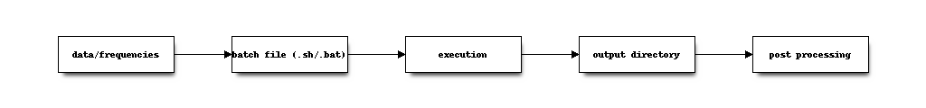
Given one or more SIP spectra in form of a frequency file and a data file, the decomposition commands could be called directly. However, given the large number of possible command line options (and environment variables), it is recommended to create a batch file with the command call. This ensures reproducability and an easier management of settings. Decomposition output is written to an output directory (in one of mulitple output formats), usually in form of human readable ASCII text files. Following that, a (limited) amount of postprocessing can be applied to the output directory.

Batch files¶

Windows¶

Windows batch files usually have the ending .bat and can be executed by a double click. Environment variables can be set using the set command. Given a functional installation of the decomposition tools, a working batch file could be:

REM This is a windows bat file, execute by double clicking on it
REM All lines starting with "REM" are comments, and will be ignored during execution.

REM environment variables are set using the syntax:
REM set [variable]=[value]

set DD_COND=0
set DD_STARTING_MODEL=3

REM the decomposition command should be globally available
REM Note that commands usually cannot span multiple lines.
REM However, using the character "^" at the end of a line indicates a multiline command.
REM Use this to structure commands for an better overview.

ccd_single -f frequencies.dat -d data.dat ^
 -n 20 -o results ^
 --tausel data_ext ^
 --nr_cores=1 --plot

Linux¶

Linux shell files usually have the file ending .sh. A typical shell file for a decomposition call is:

#!/bin/sh
# The first line indicates the program which executes this file

# comment lines start with the character '#'

# environment variables can be set using the command "export"

export DD_COND=0
export DD_STARTING_MODEL=3

# multi-line commands use the character "\" to indicate a continuation over
# multiple lines:
ccd_single -f frequencies.dat -d data.dat \
 -n 20 -o results \
 --tausel data_ext \
 --nr_cores=1 --plot

Environment variables can also be set only for a given command by prepending the assignment before the command:

DD_COND=0 DD_STARTING_MODEL=3 ccd_single -f frequencies.dat -d data.dat \
 -n 20 -o results \
 --tausel data_ext \
 --nr_cores=1 --plot

Linux shell files can be executed on the command line using the commands:

./[FILENAME].sh

or

sh [FILENAME].sh

Example: Fitting one spectrum¶

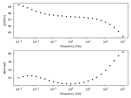
This example describes the process of fitting the following SIP spectrum using a Debye decomposition scheme:

(Source code, png, hires.png, pdf)

You need a frequency file which contains the frequencies, each in a seperate line, in ascending order:

frequency.dat (Download frequencies.dat (unix)) (Download frequencies.dat (Windows)):

Complex resistivity spectra are provided using a data file which holds a spectrum in each line. Columns are separated by space and values are linear both for magnitude and phase values. The first N columns correspond to the magnitude values ( $\Omega m$ ) corresponding to the frequencies stored in frequencies.dat. The following N columns represent the corresponding phase values.

data.dat (download data.dat (unix))

(download data.dat (Windows))

49.345594 49.120225 48.860658 48.589371 48.333505 48.113950 47.939222\
47.807051 47.709583 47.637735 47.583349 47.539704 47.501267 47.463162\
47.420588 47.368190 47.299354 47.205358 47.074354 46.890271 46.632118\
46.274900 45.794402 45.178163 44.441082 -10.526822 -12.095446 -13.004975\
-12.999086 -12.088092 -10.544173 -8.744458 -7.007706 -5.526119 -4.380307\
-3.584099 -3.124956 -2.990678 -3.184856 -3.735642 -4.701107 -6.172278\
-8.272438 -11.148023 -14.941904 -19.734922 -25.441545 -31.665354\
-37.581057 -41.99903

Note

The previous listing for the data.dat file contains only one line. For display purposes, line breaks were introduced, and indicated by ‘\’ characters.

The spectrum can now be fitted to a Debye decomposition using the command (download linux shell file) (download Windows shell file):

ccd_single -f frequencies.dat -d data.dat -o results1/

This call uses a line search to find an optimal lambda value, and saves fit results in the directory results1/.

By default, no plot is created for the fit results. The command ddplot.py creates these plots afterwards (output files are named spec_*.png:

ddplot.py -i results1/

In addition, the last iteration can directly be plotted by dd_time.py by using the option - -plot:

ccd_single -f frequencies.dat -d data.dat -o results1/ --plot

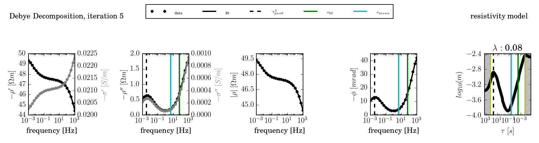
The fit can be further controlled by providing a fixed lambda value (- -lambda) and by using an advanced starting model (nr 3, using the environment variable DD_STARTING_MODEL):

Windows (download Windows batch file):

set DD_STARTING_MODEL=3
ccd_single -f frequencies.dat -d data.dat -o results2 --plot --lambda 10

Unix (download linux shell file):

DD_STARTING_MODEL=3 ccd_single -f frequencies.dat -d data.dat -o results2\
 --plot --lambda 10

_images/plot_spec_000_iteration00051.png

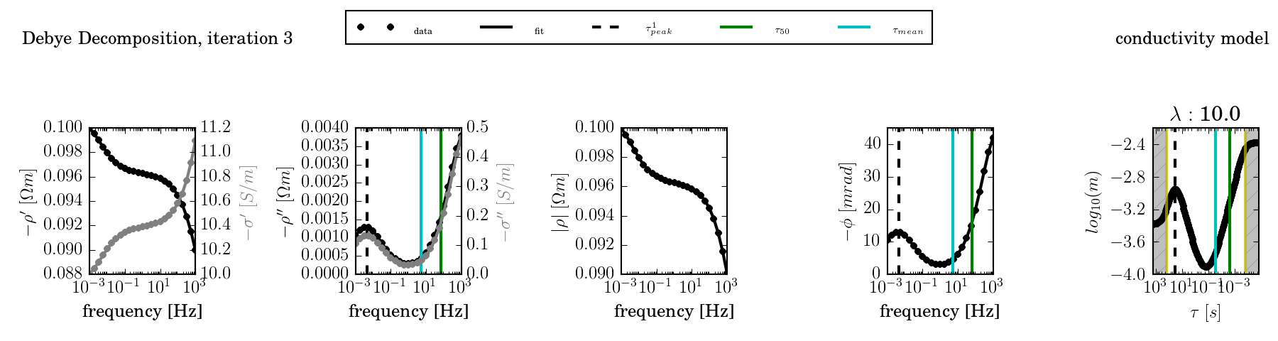
The conductivity model can be activated using the environment variable DD_COND:

Windows (download Windows batch file):

set DD_STARTING_MODEL=3
set DD_COND=1

ccd_single -f frequencies.dat -d data.dat -o results --plot --lambda 10

Linux (download linux shell file):

DD_STARTING_MODEL=3 DD_COND=1 ccd_single -f frequencies.dat -d data.dat\
 -o results3 --plot --lambda 10 --norm 10

Example: Fitting multiple spectra using a time regularisation¶

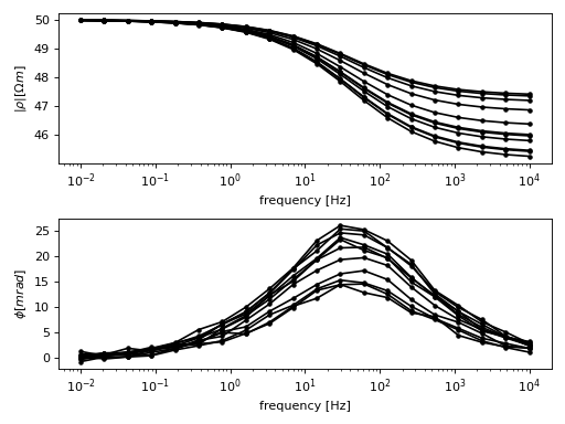
Suppose the following spectra belong to a time-lapse SIP measurement:

(Source code, png, hires.png, pdf)

Download the raw data files:

data.dat (Download data.dat (unix)) (Download data.dat (Windows))
frequencies.dat (Download frequencies.dat (unix)) (Download frequencies.dat (Windows))
times.dat (Download times.dat (unix)) (Download times.dat (Windows))

Save the files to a new directory in the subdirectory data, and rename them according to the file listing:

.
|-- data
    |-- data.dat
    |-- frequencies.dat
    `-- times.dat

To fit all spectra without any time regularisation, use the following batch file for Linux:

dd_time.py -f data/frequencies.dat\
 --times data/times.dat\
 -d data/data.dat\
 -o "results_no_time"\
 --f_lambda 50\
 --tm_i_lambda 0\
 --trho0_lambda 0\
 --plot

Use this bat file for Windows: (Download run_no_time.bat):

dd_time.py -f data/frequencies.dat^
 --times data/times.dat^
 -d data/data.dat^
 -o "results_no_time"^
 --f_lambda 50^
 --tm_i_lambda 0^
 --trho0_lambda 0^
 --plot

Important are the –f_lambda, –tm_i_lambda, and –trho0_lambda switches, which control the various regularisation strategies. For more information, please refer to the list of options for dd_time.py: ccd_time.

The resulting directory listing now should look like this (with either the .bat or the .sh file):

.
|-- data
|   |-- data.dat
|   |-- frequencies.dat
|   `-- times.dat
|.. run_no_time.bat
|.. run_no_time.sh

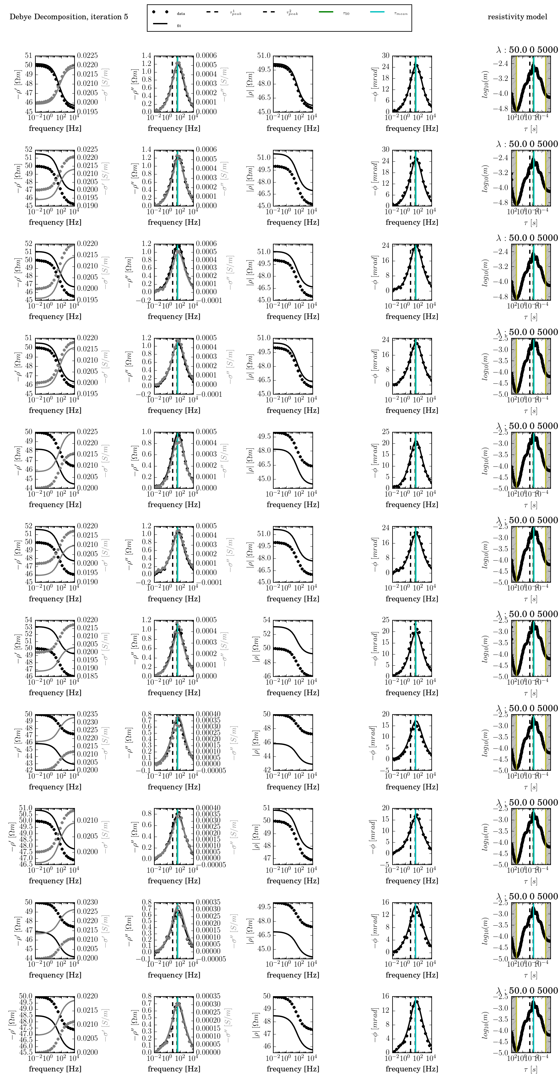
After executing the corresponding bat/batch file, results will be saved to the directory results/, with the plot file plot_times_iteration0006.png:

example2_time/results_no_time/plot_times_iteration0006.png

With dd_time.py, too, plot can be created afterward by using the command:

ddplot.py -i results1/

Getting Started¶

Workflow¶

Batch files¶

Windows¶

Linux¶

Example: Fitting one spectrum¶

Example: Fitting multiple spectra using a time regularisation¶

Time-lapse Cole-Cole decomposition routines

Navigation

Related Topics